

Table of Contents
Company Overview
Why Individual Risk Assessments Do Not Provide a Company Overview
Basic Principle
Assess Risk at the Source, Read Impact on the Business
Business Impact Analysis
The BIA as a Business Foundation
Derive Impact
Derive Impact Instead of Estimating It
Avoid Double Counting
Financial Impacts Must Not Be Counted Twice
Process Risk
From Resource Risk to Process Risk
Location and Company Risk
From Process Risk to Location and Company Risk
Concentration Risks
Identify Resource Risk Concentrations (RCR)
Time Factor
The Open Flank of Assessment
Regulation
Regulatory Compatibility
Benefits
What the Approach Achieves
Limits
What the Approach Does Not Achieve
Conclusion
Conclusion and Outlook
Sources
References and Further Sources
Organisations today assess risks in many areas simultaneously — yet still do not obtain a reliable overall picture. This article describes an approach that methodically combines the Business Impact Analysis and risk assessment: The impact of a resource is no longer estimated but derived from the impacts of dependent processes. Subsequently, resource risks are aggregated across processes, locations, and the entire company.
Why Individual Risk Assessments Do Not Provide a Company Overview
In most organisations, there are numerous risk assessments. IT systems are checked for cyber risks, technical facilities for failure risks, locations for physical threats, and suppliers for supply chain risks. In parallel, Business Continuity Management conducts a Business Impact Analysis (BIA) to determine which business processes are time-critical, what impact an interruption would have, and what resources are needed for recovery.
Both perspectives provide valuable information. However, they often remain methodologically separate. Risk assessment asks how likely an event is and what impact it would have. The BIA asks something different: what impacts arise if a specific activity cannot be performed over a certain period.
This second perspective, in particular, contains information crucial for assessing operational risks. The BIA identifies time-critical processes, MTPD and RTO, financial and non-financial impacts, as well as the required resources and their dependencies. ISO/TS 22317:2021 specifies these as the outcomes of a BIA: the assessment of the impact of a disruption over time, the determination of MTPD and RTO for prioritised activities, and the identification of necessary resources, including their dependencies.
The approach described here addresses this interface. Instead of conducting BIA and risk assessment as two separate analyses side by side, their results are combined: The BIA provides the business consequence, the risk assessment the threat — and the aggregation brings both together across process, location, and company.
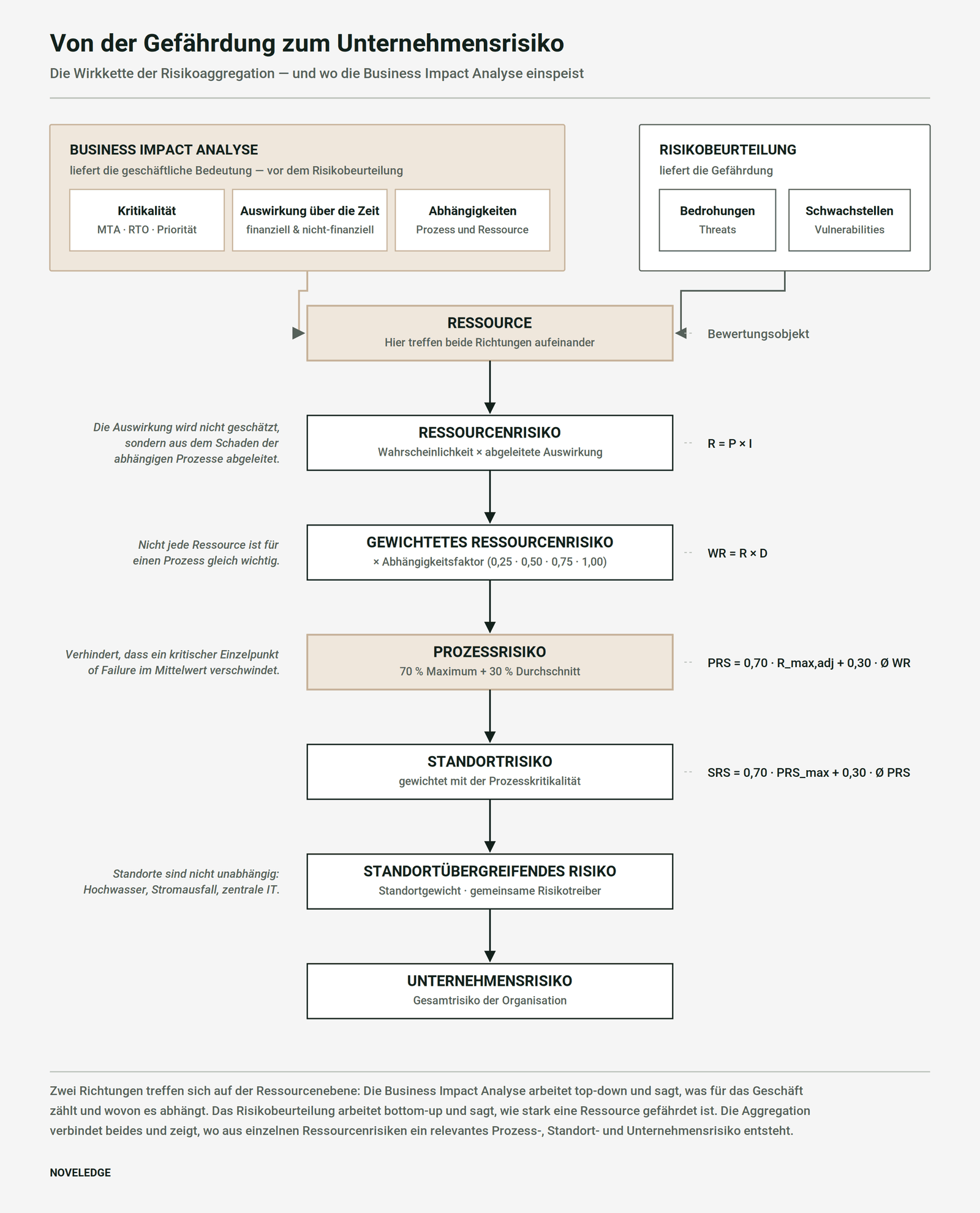
The Basic Principle
Assess risk at the cause, read impact on the business
The core methodological idea can be summarised in one sentence: The risk is assessed at the level of its cause, but its business significance is derived from the dependent processes.
A resource in itself has no economic impact. The failure of a server does not cause damage because the server has a certain acquisition value. The business damage arises because the server supports a production process, a logistics function, or invoicing.
This results in two directions that converge at the resource level:
- Bottom-up (risk aggregation): Threat and vulnerability → Resource → Process → Location → Company
- Top-down (business impact): Company performance → Process → Resource dependency
This is the key difference compared to an isolated resource risk matrix. This evaluates resources side by side without revealing which resource risk actually affects the business.
The Business Impact Analysis as a Business Foundation
The BIA therefore precedes the resource-related risk assessment both in terms of timing and methodology. It determines which processes are relevant and particularly time-critical for the organisation, and collects, among other things, MTPD, RTO, and possibly RPO, the impacts of a disruption over different time intervals, financial, regulatory, and contractual consequences, reputational and customer effects, as well as the necessary resources and their internal and external dependencies.
This sequence is also normatively plausible. ISO 22301:2019 addresses BIA and risk assessment in section 8.2 as two components of the same step: section 8.2.2 governs the BIA, section 8.2.3 the risk assessment. Both are designed to be complementary, not alternative.
Thus, the BIA already creates a relationship model between processes and resources — and in reverse reading direction between a resource and all processes that depend on it. This exact relationship model is then used for the risk assessment.
Not every resource is equally important for a process
A central piece of information is the dependency factor. It describes how strongly a process depends on a particular resource and is managed in four levels:
| Dependency Level | Factor | Significance |
|---|---|---|
| 1 | 0.25 | low dependency; the process essentially continues |
| 2 | 0.50 | noticeable restriction, but manageable |
| 3 | 0.75 | significant restriction of the process |
| 4 | 1.00 | without this resource, the process is not feasible |
The Core
Derive the impact instead of estimating it
Why estimating the impact fails in practice
In many risk assessments, those responsible must evaluate both the probability of occurrence and the impact. When it comes to financial impacts, this regularly leads to a dead end. An information security officer, responsible person, or technical manager can usually assess the threat to a server very well. However, they generally cannot reliably answer the question of what financial damage its failure would cause.
To answer it, they would need to know which business processes depend on this server, the economic significance of these processes, when their interruption becomes critical, what alternatives exist — and whether the same economic effect has already been captured by another dependent process. The result is a high data collection effort and estimates that are not comparable between evaluators.
How the derivation works
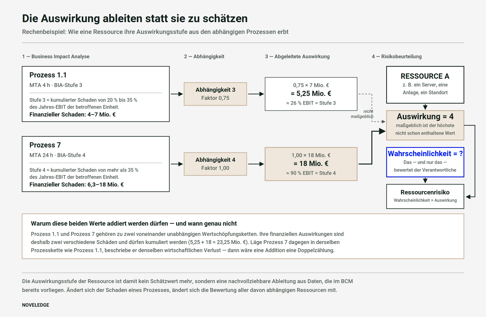
The financial damage of a resource is not estimated in isolation but derived from two already available pieces of information: the financial damage of the dependent processes from the BIA and the strength of the dependency. For a resource a and a process p, the following applies:
Damage of the Resource = Damage of the Process × Dependency Factor
Thus, a resource inherits the damage of the process on which it depends.
The following graphic illustrates this with a calculated example. It is based on an organisational unit with a planned annual EBIT of 20 million euros and a BIA matrix where level 3 corresponds to a cumulative damage of 20 to 35 percent and level 4 to damage of more than 35 percent of this EBIT.
What changes for those responsible
From Risk = estimated probability × estimated impact it becomes Risk = assessed probability of failure × derived business impact. The responsible person thus essentially only assesses one question: How likely is it that this resource will fail in the considered scenario? This brings several advantages at once:
- Consistency: The same process impacts lead to comparable resource evaluations across the organisation.
- Traceability: Every impact value has a documented derivation instead of an estimation.
- Less Subjectivity: No one has to assess financial impacts for which they lack information.
- Efficiency: Existing BIA data is reused instead of being newly collected.
- Currency: If the damage of a process changes, the evaluation of all dependent resources changes automatically.
Above all, the technical risk is directly linked to its significance for the core business. However, this requires complete information about relationships between resources and processes, process dependencies, and continuous process chains. Where this data basis is lacking, the model does not deliver better results than an estimate — only with greater effort.
The Pitfall
Financial impacts must not be counted twice
When the impact is derived from process data, a problem arises that is regularly overlooked in practice. A resource often supports multiple processes. If the BIA assigns a financial loss to each of these processes, it seems logical to add these values. This is often incorrect.
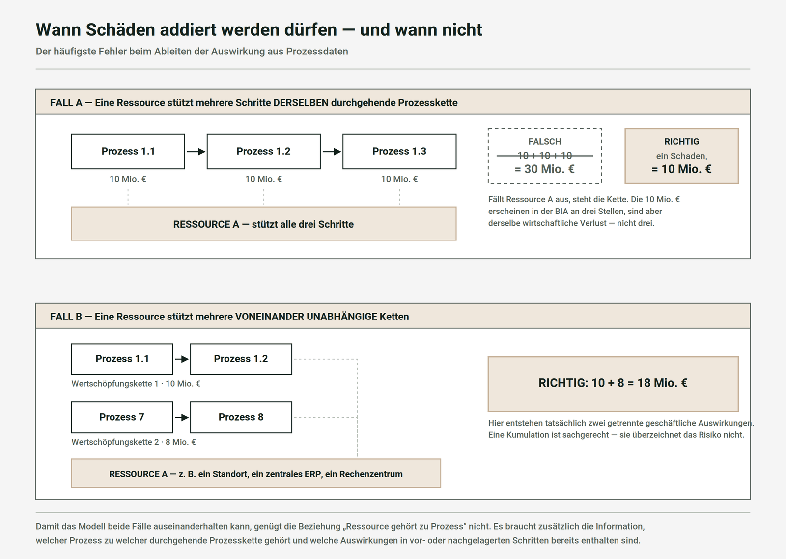
Case A
Multiple steps of the same continuous process chain
If a resource supports multiple steps of a continuous value chain, their financial impacts usually describe the same loss. A production loss of 10 million euros does not become 30 million euros just because it is visible at three points in the chain. In this case, the damage should generally only be considered once — the total damage of the chain or the highest additional damage not yet included is decisive.
Case B
Multiple independent chains
The situation is different when a site, a data centre, or a central ERP system supports multiple independent value chains. Then, indeed, several independent business impacts arise, and accumulation is appropriate.
For a system to distinguish between both cases, the relationship between resource and process is not sufficient. It also requires the assignment of each process to its continuous process chain and information on which impacts are already included in preceding or subsequent steps.
A note on the reference size, which is easily overlooked in practice: The impact is measured as a share of the planned annual EBIT, but the damage is not limited by this EBIT. If a process fails, the contribution margin is missing while fixed costs continue. Additional damages such as penalties, overtime, replacement procurement, restart costs, or customer attrition may also occur. An example: With 200 million euros in revenue, 20 million euros EBIT, and a 40 percent contribution margin, each day of downtime costs around 0.2 million euros in contribution margin — about one percent of the annual EBIT, even though only about 0.05 million euros EBIT is attributable to one day. The longer the downtime lasts, the larger the share becomes; beyond the MTPD, consequential damages usually grow disproportionately. A value over 100 percent then means that the annual result becomes negative.
If the impacts are also accumulated over independent chains, the sum can also mathematically exceed 100 percent. This is not a calculation error but a reason to examine the reference size — particularly whether the percentage levels refer to the EBIT of the affected unit or the entire company. Which financial metrics are suitable as a reference size and which are not is compared in the article on financial resilience.
From Resource Risk to Process Risk
Once the impact is derived, it is combined with the resource’s probability of failure to form the resource risk. The model uses a four-by-four matrix of failure probability and impact, the result of which is referred to as risk potential. The resources themselves can be categorised — personnel, IT, OT, location and infrastructure, products, as well as suppliers and other third parties — and the assessment is explicitly also intended at the level of entire resource groups.
Why resource risks are not simply summed up
Suppose Process A requires five resources and Process B requires twenty-five. A simple sum would assign Process B a higher risk solely because it depends on more resources. Therefore, an average is taken over the number of resources. For each resource i, the following applies:
weighted risk = risk value × dependency factor
Average = sum of all weighted risks ÷ number of resources
This step is referred to in the model as normalisation. Strictly speaking, it involves averaging, which makes processes of different sizes comparable — not normalisation to a fixed value range. This clarification of terms is more than cosmetic: it determines whether the results are later read as key figures or as index values.
Why the Average Alone is Not Enough
A pure average has a dangerous characteristic for business continuity: it averages out critical individual resources. A process with ten non-critical resources and one highly critical one appears harmless on average — even though this one resource can bring the process to a halt.
The Mixed Methods
70 Percent Maximum, 30 Percent Average
The model therefore combines both perspectives:
Process Risk = 0.70 × Highest Weighted Risk + 0.30 × Average
The peak counts more than the breadth, but the breadth is included.
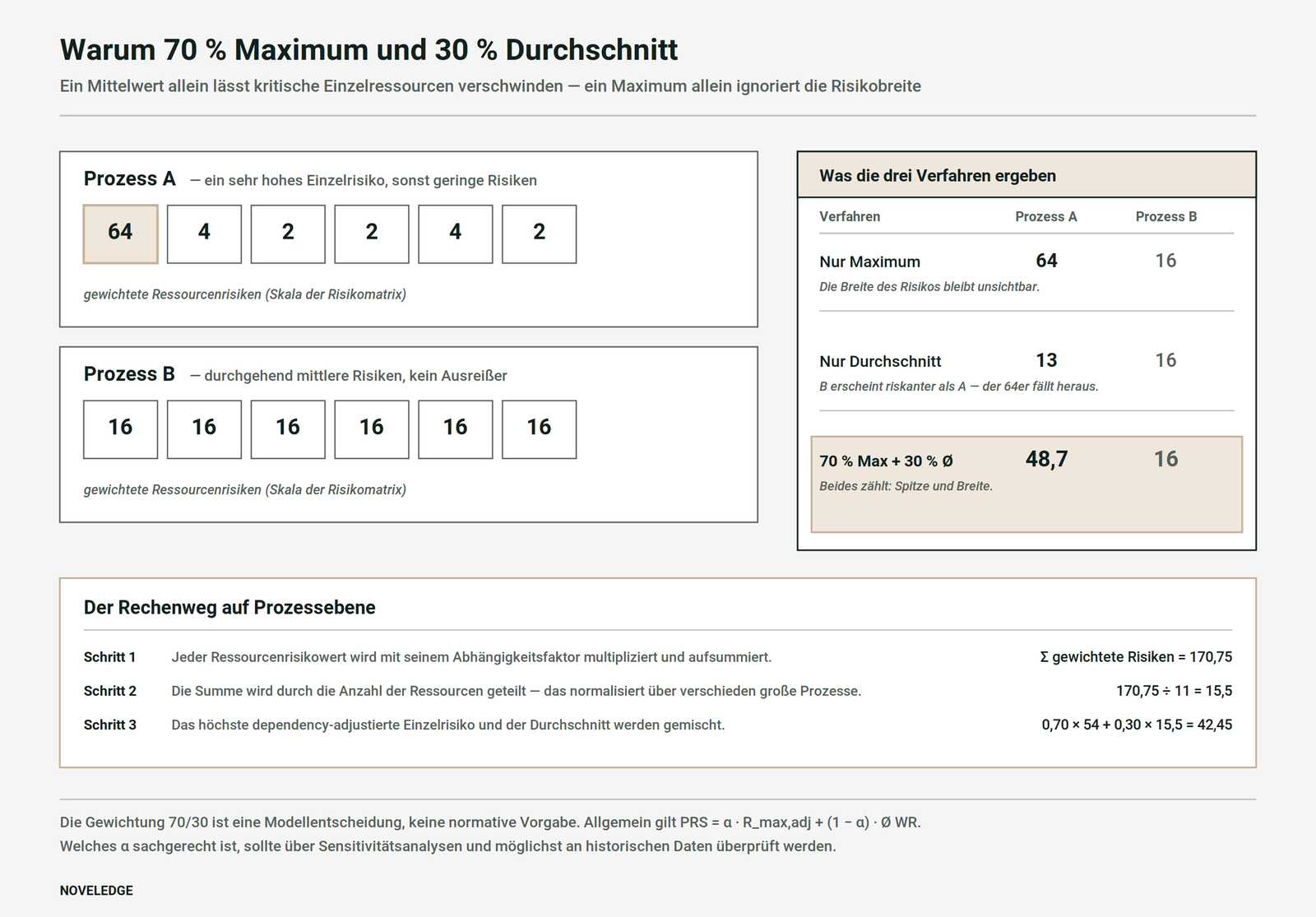
A calculated example at the process level: A process depends on eleven resources, whose weighted risk values sum up to 170.75. The average is thus around 15.5. The highest dependency-weighted individual risk is 54. This results in a process risk of 0.70 × 54 + 0.30 × 15.5 = 42.45, approximately 42.
Why Exactly 70/30?
At this point, professional integrity is more important than persuasiveness: the weighting of 70 to 30 is not a normative requirement, but a model decision. Its logic is that a highly dependent critical individual resource should not be levelled out by a multitude of smaller risks, but the overall risk exposure of a process should still be included. Generally formulated, the following applies:
Process Risk = α × Highest Weighted Risk + (1 − α) × Average with 0 ≤ α ≤ 1
The current parameterisation is α = 0.70. Which value is appropriate should be verified through sensitivity analyses and, where available, historical disruption data. Until this is done, α is a justified assumption — no more, but also no less.
For Self-Calculation
How much these settings affect the result is difficult to claim and easy to demonstrate. In the following calculation model, all variables that a Business Impact Analysis collects are adjustable: the impact progression over the downtime, the reference size, the threshold levels, the dependency factors, and the failure probabilities of the resources. The slider for α shows immediately what happens when only the average or only the maximum counts.
Alle Größen, die eine Business Impact Analyse erhebt, sind hier einstellbar. Jede Einstellung ist kurz erklärt; die Vorbelegung ist ein Beispiel und darf überschrieben werden.
1 — Business Impact Analyse
Was ein Ausfall das Geschäft kostetDas geplante Betriebsergebnis der betroffenen Einheit für das laufende Jahr, nicht das Ergebnis eines Vorjahres. Daran wird gemessen, wie schwer ein Schaden wiegt.
Ab wann eine Unterbrechung nicht mehr hinnehmbar ist. Dient hier als Orientierungsmarke, nicht als Rechengröße.
Finanzieller Schaden je Ausfalldauer
Je länger der Prozess steht, desto größer der Schaden. Diese Werte stammen aus der BIA. Der Anteil am EBIT kann über 100 % liegen: Fixkosten laufen weiter, Zusatz- und Folgeschäden kommen hinzu – besonders über die MTA hinaus.
| Dauer | Schaden (Mio. €) | Anteil am EBIT | Stufe |
|---|
Ab wann gilt welche Auswirkungsstufe?
Der Schaden wird in vier Stufen eingeteilt — gemessen als Anteil am EBIT. Höhere Schwellen bedeuten mildere Einstufung und damit kleinere Risikowerte.
2 — Modellparameter
Wie gerechnet wirdDer Schaden dieser Dauer geht in die Rechnung ein. Die Ausfalldauer ist selbst kein Rechenfaktor — deshalb entscheidet diese Wahl über das Ergebnis.
Diese vier Faktoren übersetzen die Abhängigkeitsstufen 1 bis 4 in Zahlen. Ein Faktor von 1,00 heißt: Fällt die Ressource aus, steht der Prozess. Ein kleinerer Faktor dämpft sowohl den Schaden als auch den Risikobeitrag.
3 — Ressourcen des Prozesses
| Ressource | Ausfallwahrscheinlichkeit | Abhängigkeit | Faktor | Schaden Mio. € | Auswirkung | Risikowert | gewichtet |
|---|
Ausfallwahrscheinlichkeit und Abhängigkeit werden in Stufen von 1 bis 4 angegeben — die Ausfallwahrscheinlichkeit der Ressource schätzen Sie, die Abhängigkeit kommt aus der BIA. Alles Weitere rechnet sich daraus: Schaden = Schaden des Prozesses bei der gewählten Dauer × Faktor · Auswirkung = Stufe, die sich aus dem EBIT-Anteil ergibt · Risikowert = Wert aus der Risikomatrix · gewichtet = Risikowert × Faktor. Sandfarben hinterlegt ist die Ressource mit dem höchsten gewichteten Risiko.
Ergebnis
Was die drei Verfahren ergeben
Dasselbe Prozessrisiko, dreimal verschieden gerechnet. Die Farbe entspricht der Einstufung in der Risikomatrix.
Der Rechner bewertet einen Prozess. Trägt eine Ressource mehrere voneinander unabhängige Prozessketten, addieren sich deren Schäden — dieser Fall ist im Beitrag beschrieben und im NOVELEDGE Risikorechner über mehrere Prozesse bis zum Unternehmensrisiko durchgerechnet.
Risikomatrix
Ausfallwahrscheinlichkeit × AuswirkungWaagerecht die Auswirkungsstufe, senkrecht die Ausfallwahrscheinlichkeit — beide von 1 bis 4. Der Punkt in einer Zelle zeigt, dass dort Ressourcen liegen; die Ziffer nennt ihre Anzahl.
Prozessrisiko über die Ausfalldauer
nach dem eingestellten ModellDie Kurve zeigt, welches Prozessrisiko sich ergäbe, wenn die jeweilige Ausfalldauer unterstellt wird. Solange die Dauer nicht Teil der Berechnung ist, entscheidet die Wahl eines einzigen Punktes auf dieser Kurve über das Ergebnis.
Two comparisons are particularly worthwhile. First, the threshold levels: with the preset 5 / 20 / 35 percent, a process risk of 14.3 results at 24 hours of downtime; with 5 / 15 / 25 percent, it is 21.3 — half more, without any change in the input data. Second, the scale of the matrix: switching between geometric and multiplicative gradation changes not only the numerical size but also the ratio of the risks to each other.
From Process Risk to Site and Corporate Risk
The same logic is then applied one level higher. Several processes form the risk profile of a site, and here too, neither the maximum nor the average alone would be meaningful:
Site Risk = α × Highest Process Risk + (1 − α) × Weighted Average of Process Risks
At the corporate level, the same problem arises again. Adding up all location risks would be of little use: A company with thirty locations would then automatically be riskier than one with three. Conversely, a highly critical production site must not be averaged out by twenty-nine small sales locations. Therefore, at this level, an economic or strategic location weighting should also be included — such as the EBIT or revenue contribution, the production share, or the share of critical products or services.
Locations are not independent of each other
At a cross-location level, an additional difficulty arises that simple aggregation does not capture: location risks are correlated. A flood can affect multiple locations in the same region, a cyberattack via a central IT system can impact all locations, a single supplier can affect multiple production sites, and a geopolitical event can impact an entire region.
The sum of individual location risks only becomes a reliable picture when common risk drivers and correlations between locations are considered. Methodologically, this leads from individual risk to a portfolio model. The same applies to the probabilities of failure: a power outage simultaneously causes multiple resource failures, which should not be treated as independent events.
Identifying Resource Concentration Risks (RCR)
Aggregation answers the question of how high the risk of a process, a chain, or the company is. It does not automatically answer a second question: Where do dependencies accumulate? Some resources support so many time-critical processes or such a large part of the potential damage that their failure affects the company as a whole – a central ERP system, the power supply of a location, a single supplier for a preliminary product. The NOVELEDGE Risk Calculator identifies such resources as Resource Concentration Risks (RCR). Colloquially, this is also referred to as cluster risk; the technical term in risk management is risk concentration, which can be clearly translated into English.
The fact that a resource is used by multiple processes is not sufficient for this. In a real process inventory, almost all processes share electricity, network, workplaces, and personnel. If every shared resource were considered a risk concentration, the note would appear in almost every line – and would no longer convey any information. What is meant is an unusual accumulation. The calculator checks two criteria for this and considers substitutability as an amplifier if desired.
The basis is the recorded processes. These are the time-critical processes from the Business Impact Analysis – the calculator does not include any others. „Time-critical“ is therefore not an additional selection, but the basic population.
| German | English | Abbreviation |
|---|---|---|
| Ressourcen-Risikokonzentration | Resource Concentration Risk | RCR |
| Abhängigkeitsanteil | Resource Dependency Share | RDS |
| Abhängigkeitskonzentration | Dependency Concentration | – |
| Schadenskonzentration | Impact Concentration | – |
| Substituierbarkeit / Redundanz | Substitutability / Redundancy | – |
First Criterion
Dependency Concentration
Measured is the proportion of recorded processes that depend on a resource – the Resource Dependency Share (RDS):
RDS = Number of processes dependent on the resource ÷ Total number of recorded time-critical processes × 100
If the Resource Dependency Share reaches the set threshold, a Dependency Concentration is identified. The standard value is 10%, adjustable between 5% and 50%. The 10% is an organisation-specific materiality trigger, not a universally valid or scientifically justified limit: A company with few, tightly interlinked processes will choose a different threshold than a corporation with hundreds of processes.
The Resource Dependency Share counts processes, not process chains – it measures the breadth of dependency. To make it visible whether this breadth is limited to one chain or affects multiple value chains simultaneously, the calculator additionally shows how many chains the dependent processes are distributed across. For the Resource Dependency Share, every dependency counts, regardless of the level; how significant it is, is factored into the second criterion via the Dependency Factor.
Second Criterion
Impact Concentration
The second criterion examines the total financial damage caused by the failure of the resource. For this, the calculator uses the exact resource damage it determines for the impact level, applying the same chain logic as elsewhere: The damages of dependent processes are weighted with the dependency factor. Within a process chain, only the highest damage of the chain processes (plus any additional own damages) counts, as processes within the same chain describe the same economic loss. Independent chains are added together. This damage is then related to the planned annual EBIT for the assessed downtime. The result is the consolidated EBIT loss of the resource – without double counting.
The impact level in the table is not a separate size: It is the same level as in the resource table, derived from this EBIT loss over the threshold levels. Both columns belong together. If the consolidated EBIT loss reaches the threshold, an impact concentration is identified. The standard is 30% of the planned annual EBIT. Alternatively, the threshold can be set as an impact level, for example from level 4 of the risk matrix. This value is also a setting that must fit the organisation’s risk-bearing capacity.
Amplifier
Substitutability and Redundancy
For each resource, it can be noted whether it is easily substitutable or fully redundant, only partially substitutable, or not at all (Single Dependency). This information amplifies the classification: If a resource is not substitutable and meets one of the two criteria, the risk concentration is considered critical. Conversely, existing redundancy does not lower the classification; it is mentioned in the justification, as whether redundancy holds in an emergency must first be demonstrated through exercises. A non-substitutable resource without concentration remains a Single Point of Failure for the processes that depend on it – this belongs in their risk assessment. The component can be disabled in the admin area if no reliable assessment is available.
Classification
| Status | Condition |
|---|---|
| no risk concentration | Neither of the two criteria is met – or fewer dependent processes than the minimum number. |
| risk concentration | Dependency share ≥ threshold or consolidated EBIT loss ≥ threshold. |
| critical risk concentration | Both thresholds are reached – or one threshold for a non-substitutable resource, provided substitutability is considered. |
Below a minimum number of dependent processes, neither criterion applies; the standard is 3. This lower limit complements the two thresholds for a practical reason: In small models, every resource reaches 10% with just one process. If only one process depends on a resource, a high EBIT loss is the damage of this single process – a single dependency, but not a bundling. If you do not want the lower limit, set it to 1.
Why Risk Concentration is Not Added
The resource risk concentration is a concentration indicator within the existing risk aggregation, not an additional individual risk. The damage of a concentrated resource is already included in the resource damage, its impact level, and its risk value, and from there in the process, chain, and company risk. An additional charge for concentration would count the same damage a second time. Therefore, the calculator does not change a single value when it identifies a risk concentration: It classifies and justifies.
The probability of failure is deliberately left out. Concentration describes the extent of an outage, not its frequency. Especially a rarely failing but highly concentrated resource deserves attention – in redundancy, recovery planning, and exercises. The frequency is reflected in the resource’s risk value.
Result and Example
The calculator shows for each resource: Dependency share (RDS) → dependent processes and the chains they are distributed across → consolidated EBIT loss → impact level → substitutability/redundancy → status → justification. The same table is available with the set thresholds in the PDF and Word report.
The example of the calculator includes four time-critical processes in two chains, a planned annual EBIT of €20 million, and an assessed downtime of 24 hours; substitutability is exemplarily entered for all seven resources. All four processes, distributed across both chains, depend on the ERP system: Dependency share 100%, consolidated EBIT loss 40.5%, limited substitutability – both thresholds are reached, the ERP system forms a critical risk concentration. The site’s power supply supports two processes of the same chain (dependency share 50%) with a 35% EBIT loss; with two processes, it is below the minimum number of 3. If the minimum number is set to 2, it also becomes a critical risk concentration. Only production depends on the production control system: 35% EBIT loss and not substitutable – a single dependency and a Single Point of Failure for this process, but not a concentration.
Defined Decisions
To ensure the classification remains comprehensible, the methodological determinations are summarised here:
- The German term is Ressourcen-Risikokonzentration, the English equivalent is Resource Concentration Risk (RCR). The dependency share is called Resource Dependency Share (RDS) in English; this term is not an established standard designation but the designation of this model. Abbreviations follow the English.
- The two criteria are linked with or; a risk concentration becomes critical when both are met.
- All thresholds are set values. The initial values (dependency share 10%, EBIT loss 30%, minimum number 3) are located in the admin area of the plugin and can be changed in the calculator; no number is fixed in the calculation itself.
- The population consists of the recorded processes – the time-critical processes of the BIA. There is no further selection according to the MTPD.
- The dependency share counts processes; the number of affected process chains is also indicated. Each dependency level counts.
- The consolidated EBIT loss is the resource damage of the model – once within a chain, added over independent chains. There is no second damage calculation; the impact level is derived from this.
- The reference size is the planned annual EBIT for the assessed downtime. If the duration changes, the damage concentration can change; the dependency concentration remains the same.
- A resource with fewer dependent processes than the minimum number is a single dependency, not a risk concentration.
- Substitutability and redundancy only have an amplifying effect and can be disabled.
- The probability of failure is not part of the concentration, and the risk concentration is not added anywhere.
- Regarding the classification of thresholds: Even banking supervision works with a materiality and an upper limit for concentrations – large loans must be reported from 10% of core capital and are limited to 25% (CRR, Art. 392 and 395). The figures cannot be transferred; however, the logic of a deliberately set materiality threshold can.
The Open Flank
The Time Factor
From a professional perspective, this is the most important development step still open. The BIA is inherently time-dependent. A process failure may have little impact after one hour, moderate impact after four hours, significant impact after twenty-four hours, and intolerable impact after seventy-two hours. ISO/TS 22317 describes precisely this development of impacts over time as a core result of a BIA.
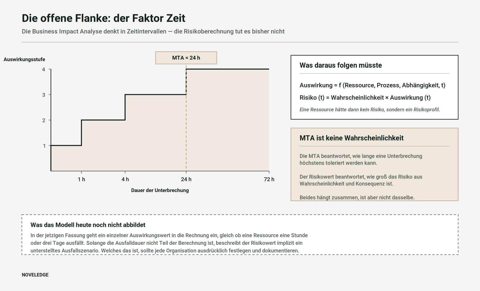
Consequently, an impact dependent on time and thus a time-dependent risk would be appropriate. The current methodology does not yet reflect this: A single impact value is included in the calculation, regardless of whether a resource fails for one hour or three days. Thus, the risk value implicitly describes an assumed failure scenario. Each organisation should explicitly define and document which scenario this is — otherwise, different areas may unknowingly assess different scenarios.
MTPD is Not a Probability
For further development, a distinction is crucial: The MTPD answers how long an interruption can be tolerated at most. The risk value answers how significant the risk is from probability and consequence. Both are related but not the same. Using the MTPD as a risk measure confuses a tolerance limit with an expectation of occurrence. Similarly, the MTPD does not limit the damage: Beyond the MTPD, it continues to grow and can exceed the planned annual EBIT.
Regulatory Connectivity
None of the relevant regulations require this specific calculation formula. It is important to note this. However, the approach operationalises requirements that several frameworks independently set.
- DORA obliges financial institutions in Article 8 of Regulation (EU) 2022/2554 to identify and document their business functions, information and ICT resources, as well as the associated dependencies and interdependencies — with a review at least once a year and after major changes.
- The CER Directive defines risk in Article 2 Number 6 of Directive (EU) 2022/2557 as a combination of the extent of a loss or disruption and the likelihood of occurrence. Article 12 requires critical infrastructures to conduct their own risk assessment, to be repeated at least every four years.
- ISO 22301 anchors BIA and risk assessment together in Section 8.2, treating them as a combined analysis step.
The added value of the model does not lie in claiming that a specific formula fulfils DORA, NIS2 or CER. It lies in establishing a quantitative link between resources, dependencies, business processes and impacts — thereby consolidating information that these frameworks already presuppose.
What the Approach Achieves
- A single source for business impact. Financial impacts are not re-estimated in BIA, IT risk management, supplier management, physical security and operational risk management.
- Consistent traceability from threat through resource, process and location to the company.
- Dependencies become computationally effective, rather than just being documented.
- Critical individual resources remain visible, because the averaging methods do not obscure them.
- A common data basis for BCM, operational risk management, Enterprise Risk Management and organisational resilience.
What the Approach Does Not Achieve
Openly Naming the Limitations
A model that conceals its limitations invites misuse. The following points are open and should be considered in every application.
- The 70/30 weighting is an assumption. It is plausibly justified, but not empirically validated.
- The dependency factors are intended to be ordinal, but are calculated cardinally. Whether a level 3 dependency should indeed weigh three times as much as a level 1 is an assumption.
- The scale of the risk matrix deserves special attention. If a four-by-four matrix is geometrically graded — for example, with values from 1 through 2, 4, 8, 16 and 32 to 64 — the result is not the arithmetic product of probability and impact, even if colloquially referred to as such. The scaling influences how strongly high individual risks dominate the aggregated result and should therefore be consciously chosen and documented.
- The duration of the outage is not yet included in the calculation.
- Continuous process chains must be clearly modelled, otherwise financial double counting threatens.
- Common causes and correlations between resources, processes and locations are not captured by simple aggregation — neither in terms of impacts nor probabilities.
- Non-financial impacts — regulatory, safety, environmental, customer and reputational effects — cannot easily be translated into euros. They should remain as separate impact dimensions.
- A score is not an expected loss. A value from a risk matrix should not be treated like a cardinal monetary amount. It ranks risks, it does not quantify them.
The thresholds for resource risk concentration are also set values. A 10% dependency share, 30% EBIT loss, and a minimum of three processes are baseline values that must fit the size of the process inventory and risk-bearing capacity. Furthermore, the dependency share is only as meaningful as the completeness of the recorded inventory: if processes are missing, the shares of the remaining ones increase.
Conclusion and Outlook
The real strength of the approach does not lie in a single formula. It lies in the fact that the Business Impact Analysis ceases to be an isolated BCM survey and becomes the data basis for translating operational dependencies into a company-wide risk picture.
The information flows in both directions. The BIA indicates what is important for the business and what it depends on. The risk assessment indicates how vulnerable these resources are. The aggregation connects both and shows where individual resource risks become relevant process, location, and company risks.
From our perspective, five questions are at the forefront for further development: the clean deduplication of financial impacts in continuous process chains, a time-dependent impact function, the handling of 1:n and n:m dependencies, the mapping of regional and cause-related correlations, and the question of whether the maximum should continue to be decisive at the location and company level or whether a high percentile would be the more robust choice.
Sources
- ISO 22301:2019 — Security and resilience. Business continuity management systems. Requirements. Section 8.2 (Business Impact Analysis and Risk Assessment). iso.org
- ISO/TS 22317:2021 — Security and resilience. Business continuity management systems. Guidelines for business impact analysis. iso.org
- ISO 31000:2018 — Risk management. Guidelines. iso.org
- Verordnung (EU) 2022/2554 (DORA), insbesondere Artikel 8. eur-lex.europa.eu
- Richtlinie (EU) 2022/2557 (CER-Richtlinie), insbesondere Artikel 2 Nummer 6 und Artikel 12. eur-lex.europa.eu
- Richtlinie (EU) 2022/2555 (NIS-2-Richtlinie). eur-lex.europa.eu
- Verordnung (EU) Nr. 575/2013 über Aufsichtsanforderungen an Kreditinstitute (CRR), Art. 392 (Definition eines Großkredits) und Art. 395 (Obergrenze für Großkredite). eur-lex.europa.eu